Group Proj placeholder

This project was done back in 2019-2020 as part of a national competition. TL;DR: you can get a robot to walk fairly robustly with periodic neural networks about 100x smaller than their non-periodic eqivalents.

Inspiration

The idea behind the neural network architecture comes from two biological concepts, which suggest something very interesting: walking can be expressed as a low-dimensional sum of periodic signals.

Central Pattern Generators

In both vertebrate and invertebrate animals, neural signals of a periodic nature are controlled by a particular type of neural circuits known as central pattern generators (CPGs). They govern respiratory and vegetative processes (breathing, chewing, swallowing, gut movements) as well as locomotion (walking, crawling, swimming, flying) in most animals and heartbeat in some invertebrates. Their main characteristic is the ability to generate rhythmic outputs from non-rhythmic inputs.

Such constructs are also used for the control of walking robots, where the CPGs are based on coupled nonlinear oscillators such as Van der Pol oscillators, which converge to a stable periodic motion and thus they ensure stable motion regardless of the initial state. The robots I’ve seen using them are usually sensorless, with the non-rhytmic input being just time. They can still yield some impressive results - one of the fastest small quadrupeds, EPFL’s Cheetah-Cub, used 1 oscillator per joint for great effect.

Kinematic Motion Primitives

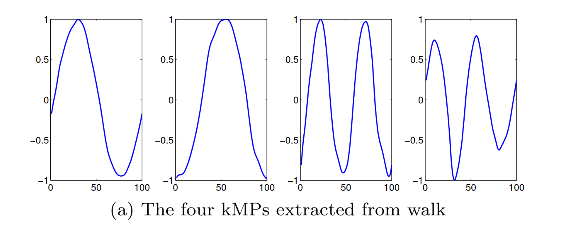
It turns out that complex movements performed by animals can be expressed as periodic signals with reduced dimensionality referred to as Kinematic Motion Primitives (kMPs). As this paper by Moro et al. shows, using principal component analysis applied to the joint data of a walking horse shows that 4 particular signals are enough to account for 97% of the variance in the joints in motion.

After those kMPs are extracted, joint trajectories for a robot with different properties were derived from them by packing them up in a vector, multiplying them by a weight matrix and adding an offset vector. Pretty similar to a linear neural network layer. The resulting gaits were again deployed on Cheetah-Cub to great effect. But let’s take a look at those KMPs for a second:

Interesting. They turn out to be pretty close to sines with varying frequencies. This seems to suggest that maybe you could get some pretty good walking from linear combos of sines.

In short, we have 2 controllers which produce fairly good results with a few periodic signals. One of them gets such results by practically plugging the signal in a single-layer linear neural net. I don’t have a horse in a mocap suit on hand… but those signals resemble sines a lot.

What if I train a neural network with a sine activation function to linearly combine a bunch of sine signals?

Software

The approach to seeing what a tiny network that does periodic signals can do was to train it in simulation using CMA-ES and then just transfer that to the real world.

Neural net architecture

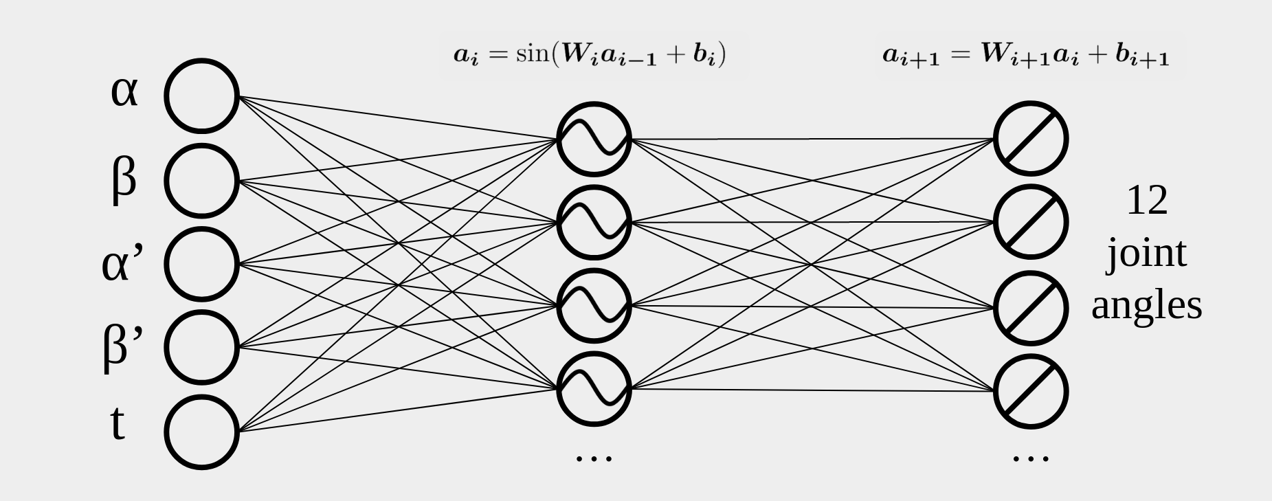
I just used a simple feedforward neural network with the following structure:

The inputs are just the IMU pitch and roll, the angular velocities in the same axes and time (to make the sine oscillate in the first place). We can modulate the sine frequency and phase in the sine layer, and its amplitutde and offset in the linear layer, meaning the training algorithm can fully modulate the oscillation.

Training algorithm

Since the networks I would be running did not have that many parameters, I settled on using CMA-ES, which has been used on some pretty difficult environments before. The behavior of CMA-ES can be described in the following manner for a problem with \(n\) parameters (in our case, the weights and biases of the network) and a population of \(\lambda\):

• In every generation, \(\lambda\) vectors are sampled, each composed of \(n\) elements: \(\boldsymbol{x}_k^{g+1},k\in(1,\ldots,\lambda)\). These vectors with parameters are taken from a multivariate normal distribution \(\mathcal{N}(\boldsymbol{m}^g,\boldsymbol{C}^g)\), where \(g\) is the present generation, \(\boldsymbol{m}^g\) - the mean of the distribution, and \(\boldsymbol{C}^g\) - the covariance matrix:

• After all rollouts of a generation have been completed, \(\mu\) of the best performing vectors are selected for calculating the new mean \(\boldsymbol{m}^{g+1}\), where \(w_i\) is the normalised reward, for which \(\sum_{i=1}^{\mu}w_i=1\):

• After that, the covariance matrix is recalculated using the mean of the present generation, which results in a matrix skewed towards the direction of the best performing solutions:

The result of all this math is that the area of possible solutions gets squished in the most promising direction, as shown in the excellent animation by David Ha. The blue dots are all vectors, the red dot is the best performing vector \(\boldsymbol{x}\), the green dot is the mean \(\boldsymbol{m}^{g}\) and the purple dots are the top \(\mu\) vectors. The objective is the global maximum, denoted by the white area:

For more explanations of other evolution strategies involving a simple 2D use case, make sure to visit David Ha’s blog.

The hyperparameters that must be specified are just the standard deviation of the first generation \(\sigma\) and the population size (the original paper provides recommended values for the rest of the hyperparameters). This algorithm possesses a relatively big time complexity (\(O(n^2)\)), but the evaluation of the population takes much more time than the covariance matrix calculation, which combined with the small number of parameters of the network (due to the small number of neurons) means that this task is suited for CMA-ES optimisation.

As described above, CMA-ES needs some sort of a reward function to evaluate how well a particular set of parameters does. This brings us to:

Reward Function

At first, I tried just using the distance travelled as the fitness function, but was having trouble with the robot just falling forwards:

This local maximum was likely due to the low motor torque making walking fairly difficult, resulting in the robot just maximising the initial reward. The reward function needed to be something incentivising stable walking, so I used this instead:

Here \(V_{avg}\) and \(V_{max}\) represent the average and maximal velocity of the body. The significance factor \(n\) defines intuitively the balance between speed and stable motion. A higher \(n\) value causes the agent to prioritise speed, but at the expense of even motion. \(\boldsymbol{d}\) is a vector that defines the desired direction of movement and \(D\) is a reward scaling factor. As ES algorithms that take the value of the fitness of every individual instead of their ranking within a generation are affected by its magnitude, changing the reward factor can have an effect on the learning rate. \

The factor \(V_{avg}/V_{max}\) has a maximal value for motion without any acceleration, i.e. \(V_{avg} = V_{max}\). The agent will still be incentivised to learn a policy that enables it to move faster if the significance factor \(n\) is bigger than 1.

With this reward function, CMA-ES now ranks neural net parameters not just by the forward movement, but by its evenness as wel, and it had a much easier time producing walking gaits - all policies in the results used this one.

Training

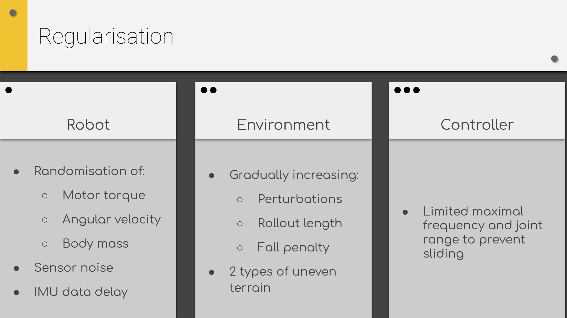
I made an URDF of the physical robot (more on this later) using the inertial data from Fusion 360 and a PyBullet-based environment compatible with the OpenAI Gym framework (this was before it was discontinued). In order to make the policy robust to the sim-to-real gap, I randomised a bunch of things, here’s the slide about them from my presentation on the project:

For most of them, the idea came from this paper by Tan et al. (I think this is where ‘sim-to-real’ came as a term too). After about 600 generations (at which point the robot can somewhat walk), the simulation applied forces of 70-100 N as perturbations that would tip the robot over unless it regains its balance. Finally, the knee joint range and maximal frequency had to be limited to prevent the robot sliding across the terrain by vibrating:

During training, I was running 6 parallel simulations using multiprocessing.Pool, 1 for each core of my laptop. It took between 1000-2000 generations to create working gaits, which was about a night of training on my Acer Aspire 7.

Sim Results

The robot managed to learn a perturbation resistant rough terrain gait. A fun little emerging behaviour is that the robot stops and takes half a step backwards if it’s stuck on an obstacle it can’t cross. Here the network uses just 8 neurons:

Adding the yaw as an input and bumping the neuron count to 12 even allowed the robot to do slight corrections to its course:

Hardware

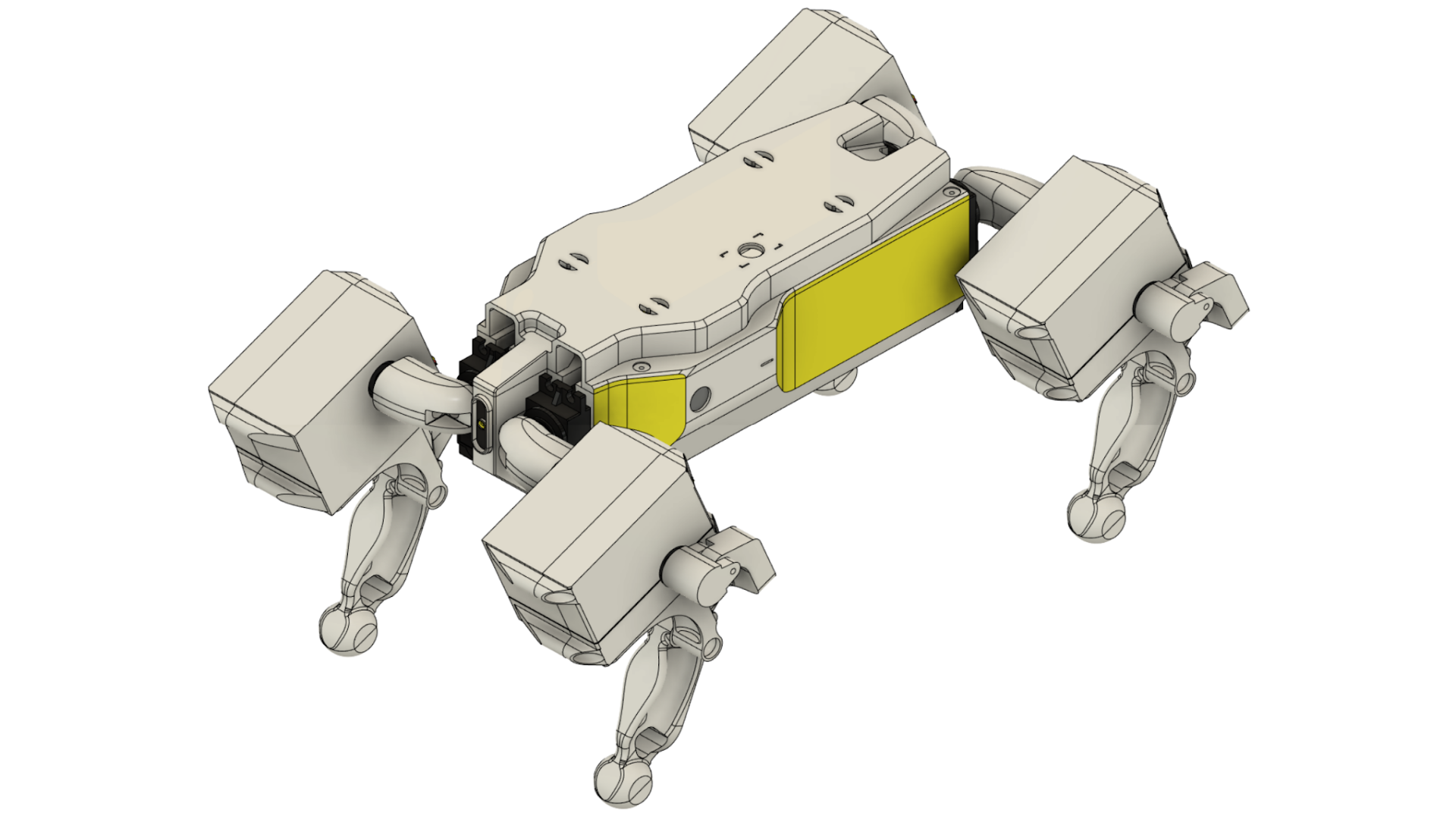
The quadruped was built with the intent to make it easy to train, meaning stubby legs and dividing it into homogenous segments to save on URDF objects and thus give my laptop at least some chance of surviving the training process. There were some cute details to it, like the slots on top for cables for a harness that never got built, the fairly clean cable management, and the fact that all screws are easily accessible.

The design did have some problems though. The desire to have the hip and knee servos together resulted in a weird curved four-bar arm which had some undesirable compliance. The legs could have been simpler too. I generated the parts for them using topology optimisation with a symmetry constraint and about 5 load cases from different directions. However, Fusion 360 outputs a mesh rather than a solid object, leading to some lofts which should’ve resulted the revocation of my education license. At least the topology optimisation resulted in geometry that I can now evaluate as ‘making sense’ - most mass was distributed away from the neutral bending axes, meaning they were fairly stiff (aside from the four-bar arm). Still, all these lessons were quite useful for future projects.

As for electronics, I used Hitec HS-645MGS for actuation, a Teensy 3.5 for the brains and a BNO055 IMU for sensing, all powered by a 2S Li-po connected to a 20A SBEC for powering everyting at a consistent 5V.

All electronics were powered to the SBEC for power using a custom PDB with a neat safety feature. The SBEC came with dual output leads, each of which ended with a generic 3-pin servo connector with a power, ground and an empty slot. I had the PDB power input pins next to each other, with the empty pins on both ends. If one connector was flipped, only a single wire would be connected to a pin and the circuit will remain open, meaning it’s not possible to short the circuit and brick everything.

Sim-to-real

I plugged the weights and biases of the rough-terrain policy in an Arduino implementation of the net. The code ran quickly enough to match the PyBullet step frequency (240 Hz), which is important as simulation-trained NNs are very sensitive to latency(as described in the Tan et al. paper). Here’s the end result deployed on the robot:

The controller showed a pretty funny case of overfitting - since the simulation spawned the robot slightly above the ground each time, it learned to somehow use the downward acceleration as a signal to start walking. This meant I had to give it a bit of velocity downwards to do so, but it still walked fine otherwise, for something with no sim-to-real adjustments. For comparison with the state of the art back then, a conventional neural netwrork needs 2 hidden layers of 125 and 89 neurons respectively after hyperparameter optimisation. The policy you are seeing here used 8.

What’s next

Nothing right now, as this was done a while ago. The robot lived a fulfiling life entertaining friends and house guests until it was scavenged for its electronic components for various other robots. As for the sine NNs, it would be good to further explore what they can do. Maybe at some point in the future.